Order of Accuracy

Theory and analysis

Posted by Sourabh Bhat on Dec 10, 2019

In this article

1. Introduction

The truncation error of a numerical method is dependent on the grid spacing. That is, every time we reduce the grid spacing (cell size), the truncation error is expected to reduce. This can be observed theoretically by carrying out a Taylor's series expansion of the numerical scheme and subtracting the result from the exact partial differential equation. The residue left out is the truncation error, which can be written as,
$$ \epsilon=c_{0}\left(\Delta x\right)^{\mathcal{O}}+c_{1}\left(\Delta x\right)^{\mathcal{O}+1}+c_{2}\left(\Delta x\right)^{\mathcal{O}+2}\dots $$
(1)
where, \(c_{i};\ i=0,1,2\dots\) are coefficients which are independent of cell size. Neglecting the higher order terms (since \(\Delta x\) is small), we get,
$$ \epsilon\approx c_{0}\left(\Delta x\right)^{\mathcal{O}}\implies\epsilon\propto\left(\Delta x\right)^{\mathcal{O}} $$
(2)
The order of such a scheme is said to be \(\mathcal{O}\) . It may not be always possible to carry out a theoretical analysis of a non-linear method, such as in the case of SDWLS, WENO or limiter based methods. In such schemes the formulation is dependent on the solution and thus, a priori Taylor's series expansion is not possible. This calls for a numerical approach for obtaining the order of accuracy of the scheme. To carry out the numerical analysis, of order of accuracy, we can write equation eq. (2) for two cell sizes, say \(\Delta x_{1}\) and \(\Delta x_{2}\) and the corresponding errors as \(\epsilon_{1}\) and \(\epsilon_{2}\) . This results in the following two equations,
$$ \epsilon_{1}\propto\left(\Delta x_{1}\right)^{\mathcal{O}} $$
(3)
$$ \epsilon_{2}\propto\left(\Delta x_{2}\right)^{\mathcal{O}} $$
(4)
Now, dividing equation eq. (4) by equation eq. (3) results in the following equation,
$$ \begin{align}&\frac{\epsilon_{2}}{\epsilon_{1}}=\left(\frac{\Delta x_{2}}{\Delta x_{1}}\right)^{\mathcal{O}} \\\implies&\log\left(\epsilon_{2}\right)-\log\left(\epsilon_{1}\right)=\mathcal{O}.\left(\log\left(\Delta x_{2}\right)-\log\left(\Delta x_{1}\right)\right)\end{align} $$
(5)
Rearranging this equation, we get an expression for the order of accuracy as,
$$ \mathcal{O}=\frac{\log\left(\epsilon_{2}\right)-\log\left(\epsilon_{1}\right)}{\log\left(\Delta x_{2}\right)-\log\left(\Delta x_{1}\right)} $$
(6)
This can be observed as the slope of a curve on a log-log plot of error versus cell size. It may be noted that the \(\Delta x\) is a measure of the cell size, and for a two-dimensional Cartesian mesh it is appropriately defined as,
$$ h=\sqrt{\Delta x\,\Delta y} $$
(7)
In case of unstructured mesh, the measure of cell size is defined by the average of all the cells in the domain, which can be defined as,
$$ h=\sqrt{\frac{\text{area of domain}}{\text{total number of cells}}} $$
(8)
and therefore, the order of accuracy of the method for a two-dimensional problem gets redefined as,
$$ \mathcal{O}=\frac{\log\left(\epsilon_{2}\right)-\log\left(\epsilon_{1}\right)}{\log\left(h_{2}\right)-\log\left(h_{1}\right)} $$
(9)
An order of accuracy analysis is a systematic process in which the error is obtained for various cell sizes. The error versus cell size is then plotted on a log-log plot. The actual order is obtained by calculating the slope of the curve on this plot. It has been pointed out by Toro [1 Toro E.F.(2009), 3rd ed., Springer ], that the order of accuracy may not be apparent in case of non-linear schemes. It is therefore essential to carry out the order of accuracy analysis of new schemes before using them. In my work, I have computed numerically the order of accuracy of the following solution reconstruction methods: first order, Beam-Warming scheme using van Albada limiter, linear and quadratic SDWLS, third order and fifth order WENO method. The analysis has been conducted for various problems in one-dimension and two-dimensions on a structured and unstructured mesh.

2. Review of Literature

The Godunov theorem [2 Godunov S.K., Mat. Sbornik(1959) ] states that it is not possible for a linear higher order scheme, (of order two or higher), to ensure a non-oscillatory solution. It is however observed that, if there are no discontinuities in the solution then, the numerical solution obtained by a linear high order scheme is much superior compared to the first order upwind scheme. It has been a quest of many researches to circumvent the limitation imposed by the Godunov theorem to achieve an order of accuracy as high as possible. This effort has led to two classes of methods of adding non-linearity to the scheme. The two classes of methods are: the artificial viscosity methods and the total variation diminishing methods. In case of artificial viscosity methods additional non-physical, viscous like terms, are added to the scheme such that the oscillations are damped out [3 Toro E.F.(1991), Springer ]. The currently available methods in this class, have to define a coefficient which has to be tuned according to the problem. Therefore, these methods are not easily extensible to general problems. The total variation diminishing (TVD) methods include slope-limiters and flux-limiters to locally switch to a lower order, based on the local gradients. This class of methods are more general to extend to any type of problems and therefore are more widely used. Many major contributions have been made to this class of methods over the years [4 van Leer B.(1973), Springer Berlin Heidelberg ,5 Boris J.P. and Book D.L., J.Comp.Phys(1973) ,6 Book D.L., et al., J.Comp.Phys(1975) ,7 Boris J.P. and Book D.L., J.Comp.Phys(1976) ,8 Harten A., J.Comp.Phys(1983) ,9 Harten A., SINUM(1984) ,10 Sweby P.K., SINUM(1984) ,11 Sweby P.K.(1989), Vieweg+Teubner Verlag ]. Various limiters have been defined which perform identically far away from the discontinuity but change their behavior close to the region of high gradients. The limiter versus the gradient-ratio plot commonly known as Sweby plot [10 Sweby P.K., SINUM(1984) ] is used in these methods to define a limiter function. Some of the widely used limiter functions are SUPERBEE [12 Roe P.L.(1985), American Mathematical Society ], VANLEER [4 van Leer B.(1973), Springer Berlin Heidelberg ], VANALBADA [13 van Albada G.D., et al., Astronomy and Astrophysics(1982) ], MINMOD [14 Roe P.L., Annu. Rev. Fluid Mech.(1986) ].

A hybrid class of schemes closely related to TVD methods are solution dependent methods. In these methods a MUSCL-type [15 van Leer B., J.Comp.Phys(1977) ] solution strategy is used, with a linear combination of all possible solution reconstructions. MUSCL stands for Monotone Upstream-centered Scheme for Conservation Laws. These type of methods include a family of more recent methods like SDWLS [16 Mandal J.C. and J S., Applied Numerical Mathematics(2008) ,17 Mandal J.C. and Rao ,.P., Computers & Fluids(2011) ] and WENO [18 Shu C.(1997), Springer ] methods. The combination of weights is so chosen, such that it reduces the oscillations. These methods do not enforce the TVD condition explicitly, and therefore may encounter oscillations within acceptable limits. In the SDWLS method, each of the neighboring cells are expressed as a function of the cell value and derivatives, using Taylor's series expansion, about the cell's centroid. This results in a system of equations with the derivatives as unknowns. Now, this system of equations are solved for the derivatives in a least-square sense, after application of weights. The weights are inversely proportional to the variation from the central cell, thus reducing the oscillations. The WENO method uses an approach where, all the candidate stencils are reconstructed. Appropriate weights are then applied to each of the stencil solutions based on the smoothness in the stencil.

The current trends in high order methods and their need are very well reviewed by Wang and group in their article [19 Wang Z.J., et al., Int. J. Numer. Methods Fluids(2013) ]. The order of accuracy analysis of WENO methods for structured grids is performed by Balsara [20 Balsara D.S. and Shu C., J.Comp.Phys(2000) ]. The analysis on unstructured grid for WENO methods is carried out by Hu [21 Hu C. and Shu C., J.Comp.Phys(1999) ] and Liu [22 Liu Y. and Zhang Y.T., J. Sci. Comput.(2013) ]. Using the ADER approach (Arbitrary high-order DERivative Riemann problem) and discontinuous Galerkin finite element method, the analysis has been performed by Dumbser et al. [23 Dumbser M. and Munz C., Comptes Rendus Mécanique(2005) ,24 Montecinos G., et al., J.Comp.Phys(2012) ]

3. Need of High Order Methods

The goal being that we need to achieve some level of accuracy, say \(10^{-3}\) of absolute error, we may ask ourselves the following question. Are high order methods really required? or is it more efficient to solve the problem on a very fine mesh using a first order method? It is well known that a first order method will run much faster than a second order method on a given mesh. But if we keep refining the mesh until the first order method achieves similar solution as second order method, will the first order method still take lesser time? The following simple demonstration tries to answer this question by actually solving a problem on various uniformly refined grids and comparing the computational time and memory requirement. The problem being solved here is a simple advection equation eq. (10), initialized with a smooth sine function eq. (11) having a wave number of unity (see Fig. 1). The boundary conditions are periodic and thus the final exact solution after one complete cycle is same as the initial distribution. The domain length chosen is 2 ranging from -1 to +1.
$$ u_{t}+u_{x}=0 $$
(10)
$$ u_{0}=u\left(x,t=0\right)=\sin\left(2\pi x\right) $$
(11)

image
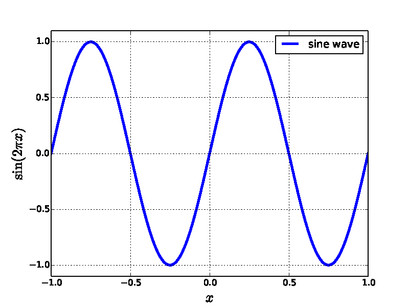
Fig. 1: Sine distribution with wave number = 1

Using a trial and error method, the number of grid cells required by the second order method is estimated. To achieve an \(L_{2}\text{-error}\) of approximately \(10^{-3}\) , the second order method requires 320 cells as seen in Table 1. Whereas, the first order method takes a phenomenal amount of cells, about 128 times more, as seen in Table 2, and therefore a proportionally large amount of memory. An even more appealing advantage of high-order methods can be observed by comparing the time taken. To achieve a similar \(L_{2}\text{-error}\) , approximately \(10^{-3}\) , the first order method takes more than 20,000 times more computational time!

Table 1: Error and computational time for Fromm (second order) method
Grid Size \(L_{2}\) Error (Absolute) Compute Time
( \(\times 10^{-3}\) seconds)
80 \(1.8518\times10^{-2}\) \(\sim20\)
160 \(4.5853\times10^{-3}\) \(\sim30\)
320 \(1.1431\times10^{-3}\) \(\sim80\)
640 \(2.8555\times10^{-4}\) \(\sim200\)
Table 2: Error and computational time for first order upwind method
Grid Size \(L_{2}\) Error (Absolute) Compute Time
( \(\times 10^{-3}\) seconds)
10240 \(5.4313\times10^{-3}\) \(\sim20000\)
20480 \(2.7209\times10^{-3}\) \(\sim300000\)
40960 \(1.3617\times10^{-3}\) \(\sim1735000\)

This overwhelming difference is observed due to two reasons. The first reason is obviously due to the higher number of mesh cells required by the first order method. The second reason is most probably the limited cache on the machine which caused repeated cache flushing. This efficiency gap between an high order method and a lower order method grows as we demand for more and more accurate results. Thus, this small experiment makes it obvious that, we must try to use higher order methods whenever possible. There are however, two major difficulties associated with high-order methods. The first difficulty is due to the oscillations which appear in the solutions. The second difficulty is associated with the stability of the methods. The TVD, SDWLS and WENO methods try to overcome these difficulties by using a non-linear solution dependent approach.

4. Results

For further reading and to look at the results using various schemes with scalar and Euler equations, download this file

5. References

[1] Toro E.F.(2009), Riemann Solvers and Numerical Methods for Fluid Dynamics: A Practical Introduction, 3rd ed., Berlin, Heidelberg, Springer, https://doi.org/10.1007/b79761
[2] Godunov S.K., "A Difference Method for Numerical Calculation of Discontinuous Solutions of the Equations of Hydrodynamics", Matematicheskii Sbornik(1959), 47, pp. 271-306, https://zbmath.org/?q=an%3A0171.46204
[3] Toro E.F.(1991), "Viscous Flux Limiters", Proceedings of the Ninth GAMM-Conference on Numerical Methods in Fluid Mechanics, pp.592-600, Springer, https://doi.org/10.1007/978-3-663-13974-4_56
[4] van Leer B.(1973), "Towards the ultimate conservative difference scheme I. The quest of monotonicity", Proceedings of the Third International Conference on Numerical Methods in Fluid Mechanics, pp.163-168, Springer Berlin Heidelberg, http://dx.doi.org/10.1007/BFb0118673
[5] Boris J.P. and Book D.L., "Flux-corrected transport. I. SHASTA, a fluid transport algorithm that works", Journal of Computational Physics(1973), 11, pp. 38-69, https://doi.org/10.1016/0021-9991(73)90147-2
[6] Book D.L., Boris J.P., Hain K., "Flux-corrected transport II: Generalizations of the method", Journal of Computational Physics(1975), 18, pp. 248-283, https://doi.org/10.1016/0021-9991(75)90002-9
[7] Boris J.P. and Book D.L., "Flux-corrected transport. III. Minimal-error FCT algorithms", Journal of Computational Physics(1976), 20, pp. 397-431, https://doi.org/10.1016/0021-9991(76)90091-7
[8] Harten A., "High resolution schemes for hyperbolic conservation laws", Journal of Computational Physics(1983), 49, pp. 357-393, https://doi.org/10.1016/0021-9991(83)90136-5
[9] Harten A., "On a Class of High Resolution Total-Variation-Stable Finite-Difference Schemes", SIAM Journal on Numerical Analysis(1984), 21, pp. 1-23, https://doi.org/10.1137/0721001
[10] Sweby P.K., "High Resolution Schemes Using Flux Limiters for Hyperbolic Conservation Laws", SIAM Journal on Numerical Analysis(1984), 21, pp. 995-1011, http://dx.doi.org/10.1137/0721062
[11] Sweby P.K.(1989), ""TVD" Schemes for Inhomogeneous Conservation Laws", Nonlinear Hyperbolic Equations — Theory, Computation Methods, and Applications, pp.599-607, Vieweg+Teubner Verlag, http://dx.doi.org/10.1007/978-3-322-87869-4_58
[12] Roe P.L.(1985), "Some contributions to the modelling of discontinuous flows", Large-Scale Computations in Fluid Mechanics, pp.163-193, American Mathematical Society, https://ui.adsabs.harvard.edu/abs/1985ams..conf..163R/abstract
[13] van Albada G.D., van Leer B., Roberts W.W., "A comparative study of computational methods in cosmic gas dynamics", Astronomy and Astrophysics(1982), 108, pp. 76-84, http://articles.adsabs.harvard.edu/pdf/1982A%26A...108...76V
[14] Roe P.L., "Characteristic-Based Schemes for the Euler Equations", Annual Review of Fluid Mechanics(1986), 18, pp. 337-365, https://doi.org/10.1146/annurev.fl.18.010186.002005
[15] van Leer B., "Towards the ultimate conservative difference scheme III. Upstream-centered finite-difference schemes for ideal compressible flow", Journal of Computational Physics(1977), 23, pp. 263-275, https://doi.org/10.1016/0021-9991(77)90094-8
[16] Mandal J.C. and J S., "On the link between weighted least-squares and limiters used in higher-order reconstructions for finite volume computations of hyperbolic equations", Applied Numerical Mathematics(2008), 58, pp. 705-725, https://doi.org/10.1016/j.apnum.2007.02.003
[17] Mandal J.C. and Rao ,.P., "High resolution finite volume computations on unstructured grids using solution dependent weighted least squares gradients", Computers & Fluids(2011), 44, pp. 23-31, https://doi.org/10.1016/j.compfluid.2010.11.021
[18] Shu C.(1997), "Essentially non-oscillatory and weighted essentially non-oscillatory schemes for hyperbolic conservation laws", Advanced Numerical Approximation of Nonlinear Hyperbolic Equations, pp.325-432, Berlin Heidelberg, Springer, https://doi.org/10.1007/BFb0096355
[19] Wang Z.J., et al., "High-order CFD methods: Current status and perspective", International Journal for Numerical Methods in Fluids(2013), 72, pp. 811-845, http://doi.wiley.com/10.1002/fld.3767
[20] Balsara D.S. and Shu C., "Monotonicity Preserving Weighted Essentially Non-oscillatory Schemes with Increasingly High Order of Accuracy", Journal of Computational Physics(2000), 160, pp. 405-452, https://doi.org/10.1006/jcph.2000.6443
[21] Hu C. and Shu C., "Weighted Essentially Non-Oscillatory Schemes on Triangular Meshes", Journal of Computational Physics(1999), 150, pp. 97-127, https://doi.org/10.1006/jcph.1998.6165
[22] Liu Y. and Zhang Y.T., "A Robust Reconstruction for Unstructured WENO Schemes", Journal of Scientific Computing(2013), 54, pp. 603-621, https://doi.org/10.1007/s10915-012-9598-3
[23] Dumbser M. and Munz C., "ADER discontinuous Galerkin schemes for aeroacoustics", Comptes Rendus Mécanique(2005), 333, pp. 683-687, https://doi.org/10.1016/j.crme.2005.07.008
[24] Montecinos G., et al., "Comparison of solvers for the generalized Riemann problem for hyperbolic systems with source terms", Journal of Computational Physics(2012), 231, pp. 6472-6494, https://doi.org/10.1016/j.jcp.2012.06.011

Beta testing note: This page is automatically generated using a tool developed by me (inspired by \( \LaTeX \)'s cross-referencing). Please report any formatting errors (or cross-referencing errors) so that it can be corrected in all posts. Thank You!

Comments / Feedback

Note: Comments will appear after review, which may take upto 24 hrs.